Maxwell’s Equations
A gentle introduction

Before we begin, be aware that talking about electromagnetism in any meaningful way means talking about vector calculus. Please don’t be intimidated, even if you don’t have the first idea what any of the symbols or terms mean. Vector calculus is hard but its core ideas are intuitive and I will explain everything as we go.
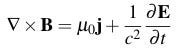
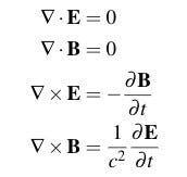
In SI units, Maxwell’s famous equations for the electric and magnetic fields are:
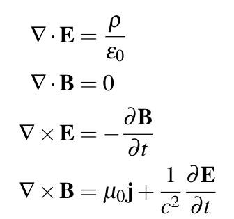
These are differential equations (equations which describe a rule for the rate of change of a function with respect to one or more of its input variables) for the electric field E and the magnetic field B in the presence of a charge function ρ (“rho”) and an electrical current j. The quantities ε₀ (“epsilon naught”) and μ₀ (“mu naught”) are physical constants called the permittivity and permeability of vacuum. The speed of light c obeys the important relation c² = 1/ε₀μ₀. When boundary conditions for the fields are specified, these equations completely and uniquely determine the fields.
Usually one does not attempt to solve these equations directly for a given configuration of boundary conditions, charges, and currents. Instead, numerous mathematical tricks have been invented to simplify many different kinds of problems. However, it is still important to understand the physics behind these equations.
The electric and magnetic fields
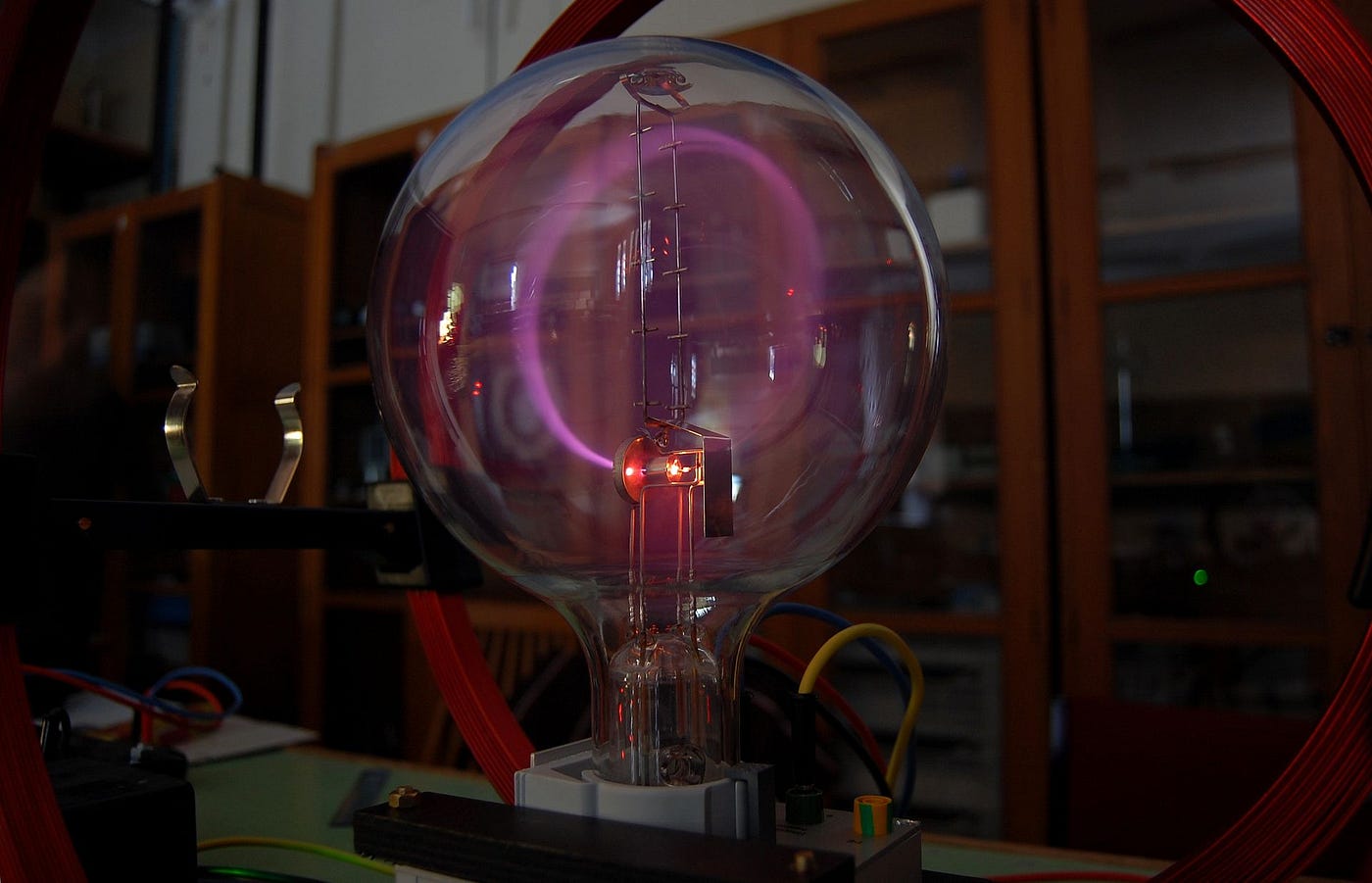
A charge q with velocity vector v and speed much less than c in the presence of an electric field E and a magnetic field B is subject to the Lorentz force:
Interestingly, this is still true in the relativistic case when the force F is meant to denote the time rate of change of the relativistic momentum instead of the classical momentum. There are two terms in the Lorentz force. The first is qE, called the electrostatic force. This force is caused by the electric field E, which is produced by stationary charges. The second force is qv⨯B, which is called the magnetic force. The symbol ⨯ is called the vector or cross product, and it denotes a vector perpendicular to v and B and with magnitude |v||B|sin(θ) where θ is the angle between v and B.

A magnetic field B is produced by a current and interacts with a moving charge to produce a force. A current is a charge times a velocity so qv is a current element, and it follows that magnetic forces act between currents.
To simplify things, we will pretend that currents and charges are separate entities that exist independently of each other. Now this obviously is not the case because a current is by definition a moving charge, but when we start talking about moving charges we have to bring in special relativity. However, we can get very far without relativity, as did James Maxwell and his contemporaries. It turns out that Maxwell’s equations are already relativistic, though the 19th century physicists couldn’t have been aware of it. A follow-up to this article will address this if there is enough interest.
So for our purposes, stationary charges exert forces on other stationary charges via the electric force and currents produce forces on moving charges via the magnetic force.
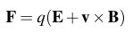
An example of the Lorentz force can be seen in the case of cyclotron motion. Suppose that a magnetic field points into this page and an electron has a velocity vector entirely in the plane of this page.
The x symbols denote a uniform magnetic field pointing into the page. The force vector, in red, is the cross product of v and B and so by the right-hand rule the force vector points towards the center of a circle. If a charge in a uniform magnetic field is given some initial velocity with a direction perpendicular to B then the charge will move in a circle at constant speed. This is called cyclotron motion.
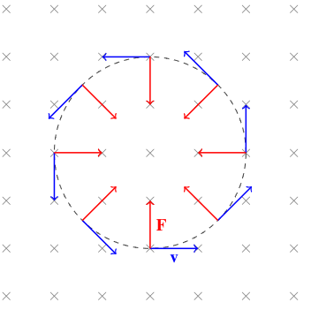
A Teltron tube (pictured above) is a device that demonstrates cyclotron motion. Free electrons are produced heating a small filament and given an initial velocity by producing an electric field in the small region around the device. The field in the tube produced by the two coils is approximately uniform, so it pulls the motion of the electrons into a ring. The electrons produce light as they strike atoms of a very low-pressure gas.
Vector fields, field lines, and flux
The electric and magnetic fields are vector fields. A vector field is a function that assigns vectors to points in space, as in the following picture which shows the electric field vectors of an electric dipole consisting of a positive charge at (+1,0) and a negative charge at (-1,0). Note that for clarity’s sake, the vectors only show the direction and not the magnitude.
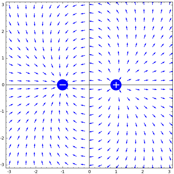
You can see that electric field vectors point away from positive charges (sources) and towards negative charges (sinks). Since the force on a positive test charge q is given by F=qE, this corresponds to the fact that charges of opposite sign attract and charges of equal sign repel. We almost always assume that the sources of the fields, be they charges or currents, do not move.
Just as important as the vectors of the vector field are the field lines. For the electric dipole the field lines probably look familiar to many of you:
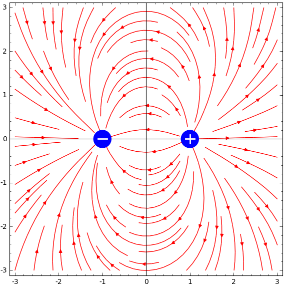
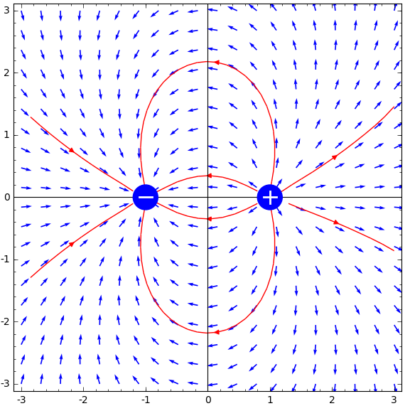
To get a clearer picture of what the field lines tell us, let’s pick out just a few of them and show them along with the field vectors:
This diagram shows some important properties of field lines.
- Field lines are not just curves in space, they also have a direction. A field line originates at a source and terminates at a sink. It may also originate or terminate at infinity. They appear to break in the pictures because of the limitations of the software I used to draw them.
- Field lines are tangent to field vectors at every point.
- Field lines never intersect each other, or else the vector at the point of intersection would be pointing in two directions at once, which is impossible.
- Field lines change their direction continuously.
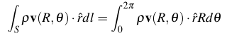
Let us now briefly change our focus from electromagnetism to fluid dynamics. Suppose that the velocity of water with uniform area density (kg/m², since we are considering a two dimensional problem) ρ around a source is given at every point by a vector-valued function v(r, θ), where r is the radial distance from the source and θ is the angle between the position vector of r and the horizontal.
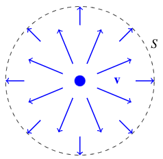
Suppose that the source is located at the blue dot, and that the boundary S is a circle of radius R. How much water flows past this boundary per second?
Dimensional analysis is always a great place to start a problem like this. We are asked for something with units of kg/s and we are given an area density with units kg/m² and a velocity with units m/s. We can combine these to get the momentum per unit area, which has units of kg/m⋅s. If we can eliminate the units of 1/m from this quantity then we will end up with something with the right units. This should make us think about integrating the quantity ρv with respect to length l along a curve C, but ρv is a vector quantity and we are asked for a scalar quantity, so we need to introduce a dot product somewhere. Since the water flows over S, we might naturally guess that the curve C should be the circle S and the vector should be the unit vector pointing out of the circle. It turns out that this is the correct approach, and the answer to the problem is the quantity
This is called the flux of the vector field v over the boundary S. The flux of a three-dimensional vector field through a surface or a two-dimensional vector field through a curve can be interpreted as telling us how much that vector field “flows” over the surface or curve. If v is any vector field and S is a boundary (surface or curve) enclosing a region (volume or area) V, then we also have the critically important divergence theorem, which we present here without proof:
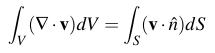
Thus the total flux over the boundary of the volume is equal to the integral of ∇⋅vwithin the volume, so we can think of ∇⋅v as the flux leaving each point within V. The quantity ∇⋅v is called the divergence of v and it is the subject of the first two of Maxwell’s equations.
Gauss’s Law

This is the differential form of Gauss’s Law. Let’s first consider the integral form. Suppose that S is a closed surface and that the total charge in the region enclosed by S is Q. Then:

So Gauss’s Law tells us that the flux of the electric field through S is the total charge enclosed by S divided by the permittivity. One of the great features of this law is that S can be any surface that completely encloses the charge distribution, and the flux through the surface will be the same.
The differential form is obtained with the divergence theorem:
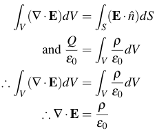
Note that in general ρ is a function of position. We will not consider the case where it is also a function of time since that would require special relativity, although the follow-up to this article might.
The differential form can be thought of as the integral form applying to infinitesimally small spheres enclosing every point in space.
Gauss’s Law tells us a few useful things:
- If ρ(x,y,z) is positive then the flux leaving point (x,y,z) is positive and if ρ(x,y,z) is negative then the flux leaving point (x,y,z) is negative, which is equivalent to saying that a positive flux enters point (x,y,z). This formalizes our earlier claim that field lines originate at positive charges and terminate on negative charges.
- If there is no charge in a region of space, then any field line that enters that region must exit that region.
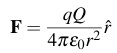
Let’s derive Coulomb’s Law as a demonstration of Gauss’s Theorem. Suppose that a point charge Q is located at the origin and a test charge q is located at a distance r from the origin. Since F=qE, this problem can be solved by finding Edue to Q. Let the Gaussian surface S be a sphere of radius r centered at the origin. Let’s start by writing down Gauss’s Law:
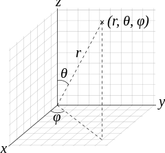
The unit vector is in the radial direction, and the differential area element dS for the surface of a sphere of radius r is r²sin(θ)dθdφ where φ and θ are as in the diagram:
Therefore:
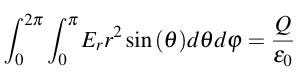
By symmetry, we can see the electric field depends only on distance from the origin so we can pull it and r out of the integral:
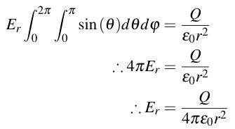
E must be radial because electric forces act on the line between two charges:
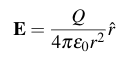
Then we obtain Coulomb’s Law with F=qE:
Gauss’s Law for magnetism

This law tells us that all magnetic fields are divergenceless. Using the ideas we developed in the last section, this means that:
- There is precisely zero net flux entering or leaving any region in the presence of a magnetic field. Any field line that enters any region must exit that region.
- All field lines form closed loops.
- There are no sources or sinks for magnetic field lines. Equivalently, we can say that magnetic charges, or monopoles, do not exist in classical electrodynamics (the jury’s still out on whether they exist in quantum electrodynamics).
The most important use of Gauss’s Law for magnetism is in defining the vector potential. That would take us beyond the scope of this article so we will just move on.
Interlude: Conservative fields
We know from basic physics that the work done on a particle when that particle is made to move a distance ∆x by a constant force F is W=F∆x. If instead F varies continuously and the particle is made to move in a straight line from a to b then the work is

What if instead the particle moves along a curve of arbitrary shape in a three-dimensional force field? Suppose that F is a force field and that the particle moves along a curve C, which may or may not form a closed loop. At any point along the curve, we can say that F is a vector with three components: one along êₙ, perpendicular to the curve, one along êₜ, tangent to the curve, and a component along êₙ⨯êₜ, perpendicular to êₙ and êₜ. Only the component of F in the direction of the path does work so we take its dot product with êₜ and integrate with respect to dl, the differential length element of the path:
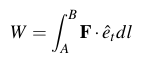
There exists a special class of force fields called conservative fields, which may be written as the negative gradient of a potential energy function: F=-∇U. If this is the case, then the fundamental theorem of calculus for line integrals tells us that:
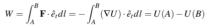
This means that for a conservative force field, the work done by a particle as it moves from point A to point B depends only on those points and not on the path chosen. In fact, this is usually given as the definition of a conservative force field, but the definition of a conservative field as a vector field arising from the gradient of a potential is exactly equivalent: a force field F is conservative if and only if we can say that F = -∇U.
It is also clear from this equation that if the particle moves along any closed curve C, then the work done is 0. We write this as:
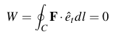
The circle in the integral sign indicates that the path of integration is a closed loop.
In addition to the divergence theorem, the other theorem you must know to get anywhere with learning electromagnetism is Stokes’ Theorem, which we present without proof. For any surface S for which C is the boundary:

From this we can also see at once another equivalent definition of a conservative field: since if F is conservative then it is the gradient of a function and since ∇⨯(∇A)=0 for any function A, we see that ∇⨯F=0 if and only if F is conservative. We can think of ∇⨯F as the tendency of a field to cause rotational motion about a point. This quantity is known as the curl of F and it is the subject of the next two of Maxwell’s Equations.
The Maxwell-Faraday equation
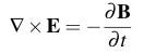
This is one of the first of two equations that connect E and B. It tells us that E is a conservative field in the absence of a magnetic field or if the magnetic field is constant in time. To interpret this, let’s start with what we know about about potential and kinetic energy.
Physical systems will evolve through time in a way that allows them to minimize their stored potential energy. They do so by transforming potential energy into kinetic energy by performing work. In a conservative force field, a particle does no work by moving in a closed loop, and so there is no way that a conservative force field can cause a particle initially at rest to move in a loop. Closed orbits can occur depending on the initial velocity, as in the case of planetary motion.
Suppose that we want a charged particle, initially at rest, to move in a closed loop. This means that we must make the electric field nonconservative, so we must give it a nonzero curl. We turn to dimensional analysis to guide our intuition. Since Ehas units of N/C, ∇⨯E has units of N/C⋅m. We know that B has units of Teslas, and 1T = N⋅s/C⋅m. Therefore ∇⨯E has units of T/s. Since ∇⨯E is a vector field, this means that we must expose a charged particle to a vector field with units of T/s if we want it to move in a closed loop.
Since the quantity -∂B/∂t is a vector field with units of T/s, it’s possible that this is the quantity that we’re looking for, and Maxwell determined that it is indeed the case that ∇⨯E=-∂B/∂t by interpreting Faraday’s experimental data.
We can use this equation to derive Faraday’s Law of Induction, which states that:
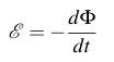
The quantity ℰ (script E) is called the electromotive force in a loop of wire and has units of volts, and 𝛷 is the flux of the magnetic field through the area enclosed by the loop. The EMF is the work done by a unit charge as it moves once around the loop, therefore:
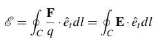
So according to Stokes’ Theorem:
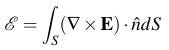
Then by the Maxwell-Faraday equation:
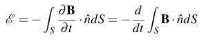
The partial derivative with respect to time gets pulled out of the integral and turned into an ordinary derivative because the integral does not depend on position. By definition, this integral is the flux of B through the area enclosed by the loop of wire C so this completes the proof that
This explains why a changing magnetic field near a circuit induces a current in that circuit.
Ampere’s Circuital Law
And finally we come to Ampere’s Law. Ampere’s Law allows us to finish the process of building a complete unified theory of electromagnetism and electromagnetic waves.
Let’s start with the original form of this law, ∇⨯B=μ₀j, which holds when there is no time dependence. This tells us that the circulation of the magnetic field around a point is proportional to the current at that point. The integral form of this equation is:
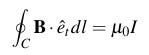
This says that the integral of B around a closed loop is proportional to the total current penetrating the area enclosed by the loop. As a demonstration, we can use this to find the magnetic field around a wire. In this case the tangent vector is in the polar angle direction and so if we put the wire at the center of an imaginary loop of radius r, then dl =rdθ. Then:
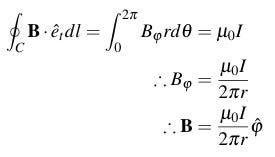
This formalizes the right-hand rule for a magnetic field around a wire:
In the time-independent case, E is always conservative because its curl is zero. But we’ve just seen that even in the time-independent case B is only conservative in a region containing no currents, and most interesting problems involve regions near current. Furthermore, the magnetic force F=qv⨯B is never conservative because it depends on velocity. So we can’t treat B as a conservative field in general, and those rare cases where we can are not important for us right now.
Now let’s talk about the second term in the right hand side of Ampere’s Law, called the displacement current. The name comes from another field, called the electric displacement D=ε₀E, which is useful in problems involving fields in materials rather than empty space. Ampere’s Law as originally written did not include this term, and it was Maxwell who discovered that it was necessary. Before then, that incompleteness in Ampere’s Law caused some problems. Most significantly, it would have meant that electromagnetic waves couldn’t exist.
In physics, a wave equation is a differential equation with the form:
The operator ∇² is called the Laplacian and it is given by:
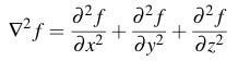
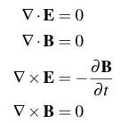
And k is the speed with which the wave propagates through space. If the function f is instead a vector field, then each component of the vector satisfies the equation. Let’s try to obtain wave equations in free space (no charges or currents), pretending to be ignorant of the displacement current. Maxwell’s equations would then be:
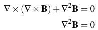
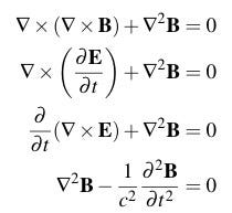
Let’s start with the vector calculus identity ∇⨯(∇⨯A)=∇(∇⋅A)-∇²A where ∇²A means that the Laplacian operator is applied to each component function of A. Since ∇⋅E=∇⋅B=0, this means that ∇⨯(∇⨯E)=-∇²E for the electric field and ∇⨯(∇⨯B)=-∇²B for the magnetic field. If ∇⨯B=0 in free space then observe that we can’t get the correct wave equations. For E we get:
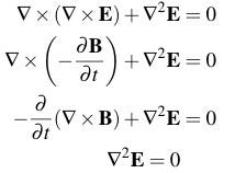
And for B we get:
To fix this, we have to add the displacement current. Of course, we can’t just plug in the displacement current because it will give us the equations that we want, we need to justify it. To do so, let’s anticipate that the problem is in the equation ∇⨯B=μ₀j. Let’s take the divergence of both sides: ∇⋅(∇⨯B)=μ₀∇⋅j. Since the divergence of a curl is always zero, this means that ∇⋅j=0 always. But this not the case. Electric currents obey the continuity equation:
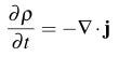
This equation says that the rate of change of the charge in a region is the negative of the net current flowing out of the region. If ∇⋅j is positive so that there is a net outflow of charge then the charge in the region must decrease, and vice versa if it is negative.
This means that we must instead have:
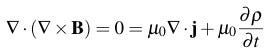
This means that ρ is the divergence of some vector field. Happily, Gauss’s Law tells us that there is a vector field whose divergence is equal to ρ, that being ε₀E, the displacement. If we plug ε₀∇⋅E in for ρ and cancel the divergence from both sides, then we get the correct equation:
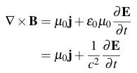
This gives us the correct Maxwell equations for free space:
Now we can get the correct wave equations:
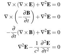
For E. Then for B:
This is why these equations are named for Maxwell even though he didn’t discover the laws that they describe. It was his ingenious idea to introduce the displacement current into Ampere’s Law that allowed for the final unification of the theory of classical electromagnetism.
Conclusion
If you managed to make it to the end of this, then you should be proud of yourself. This is pretty difficult stuff and we’ve only just scratched the surface. If there’s enough interest, then the next article will be expand on some points about relativity that I alluded to in this article. Let me know in the comments if you think I should write that. I’ll end this article with a little teaser on what that would entail.
Stinger: Covariance
The principle of covariance says that the laws of physics must appear to be the same according to all observers in the universe, in the sense that the form of the equations describing those laws must be the same in all reference frames.
Suppose that the origins of two coordinate systems S and S’ are in relative motion with constant speed V along the x-axis.
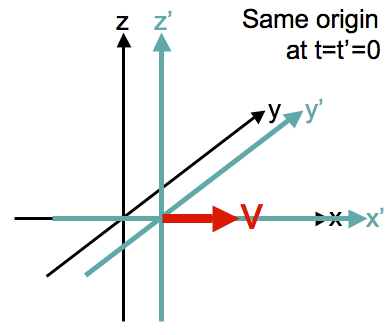
The primed coordinates are related to the unprimed coordinates by the Galilean Transform:

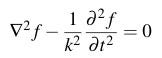
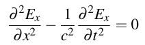
Let’s consider just the one-dimensional wave equation for the x-component of E. The principle of covariance tells us that if someone in frame S observes an electromagnetic wave and determines that the wave equation is
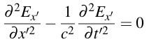
then the observer in S’ measuring that same wave must observe the equation in terms of their coordinates as
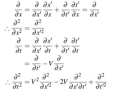
Can we accomplish this by making a Galilean transform on the coordinates? Using the transforms and the chain rule, the partial derivatives transform as:
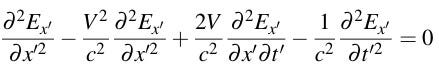
So the unprimed wave equation transforms into:
This means that there’s a problem, and it’s either the wave equation or the transformation. It can’t be the wave equation because Maxwell’s equations are verified by experiment, so the problem is with the transformation. To solve this problem, we must let go of some of our most fundamental ideas about the world and introduce special relativity.


