
Flow Characteristics of Fibrous Gas Diffusion Layers Using Machine Learning Methods


1
Forschungszentrum Jülich GmbH, Institute of Energy and Climate Research, Electrochemical Process Engineering (IEK-14), 52425 Jülich, Germany
2
Modeling in Electrochemical Process Engineering, RWTH Aachen University, 52056 Aachen, Germany
*
Author to whom correspondence should be addressed.
Appl. Sci. 2022, 12(23), 12193; https://doi.org/10.3390/app122312193
Submission received: 11 October 2022
/
Revised: 19 November 2022
/
Accepted: 25 November 2022
/
Published: 28 November 2022
(This article belongs to the Section Computing and Artificial Intelligence)
Abstract
:The material characteristics of gas diffusion layers are relevant for the efficient operation of polymer electrolyte fuel cells. The current state-of-the-art calculates these using transport simulations based on their micro-structures, either reconstructed or generated by means of stochastic geometry models. Such transport simulations often require high computational resources. To support material characterization using artificial-intelligence-based methods, in this study, a convolutional neural network was developed. It was trained with results from previous transport simulations and validated using five-fold cross-validation. The neural network enables the permeability of paper-type gas diffusion layers to be predicted. A stochastic arrangement of the fibers, four types of binder distributions, and compression of up to 50% are also considered. The binder type and compression level were features inherent to the material but were not the subject of the training. In this regard, they can be seen as features hidden from the training process. Nevertheless, these characteristics were reproduced with the proposed machine learning model. With a trained machine learning model, the prediction of permeability can be performed on a standard computer.
PACS:
88.30M-; 88.30gg; 88.30pj1. Introduction
The efficient operation of polymer electrolyte fuel cells (PEFCs) requires knowledge of the properties of all of their components, as well as the proper configuration and design of the entire system. One component of interest is the gas diffusion layer (GDL), which is typically made from fibers. The relevance of the structural characteristics of porous media was shown by Hoppe et al. [1], who visually depicted the deformation of fibrous GDLs under misaligned flow-field structures in a fuel cell assembly. Although the fibers are relevant for detailed investigations within the micro-structure of the fluid through-flow, macroscopic properties—e.g., permeability—are required for optimizations at higher scales (cells and stack), as was shown by Kvesić et al. [2] and Reimer et al. [3]. Meanwhile, Mukherjee et al. [4] investigated the role of gas permeability (through-plane as well as in-plane) on fuel cell performance. Again, the macroscopic properties of porous media can be obtained from measurements or mesoscale transport simulations. Yuan et al. [5] presented a comprehensive overview of the properties of PEFC components, whereas Yuan et al. [6] focused on GDL properties. In turn, Kaneko et al. [7] reported some variation in the diffusivities measured by different researchers. The electrochemical properties of GDLs were experimentally outlined by Syarif et al. [8].
Furthermore, these properties can be determined by means of transport simulations of the micro-structure. This was previously undertaken by the authors of [9] and fleece-type GDLs [10], as well as by other researchers [11]. Gao et al. [12] simulated gas transport in woven cloth GDLs. Although the influence of the orientation of straight fibers on gas permeability was already investigated by Tomadakis and Robertson [13], this topic remained an issue in two-phase investigations by Lee et al. [14]. All of these studies have in common the fact that they required extensive computational resources. Even more computational resources were employed by Lintermann and Schröder [15], who simulated gas flow through a fiber-based GDL using lattice Boltzmann (LB) simulations with a high degree of accuracy, operating in a hierarchical octree-based mesh.
Nowadays, methods based on artificial intelligence (AI) have been rising to the forefront of various fields of research. A prominent member of the AI portfolio is machine learning (ML). Furthermore, deep learning (DL) makes up part of the broader ML family and is based on artificial neural networks (ANNs) featuring non-trivial structures [16]. Oliveira et al. [17] acknowledged the rising significance of ML for databases on material properties, identifying an ongoing lack in several fields, some of which include energy storage and conversion. Supervised learning—again, a form of ML—employs data sets, each of which are labeled with so-called features to train an ML model. Afterwards, the ML model can be used as a black box to obtain predictions based on previously unseen features in the data. The appropriate collection of training data is crucial for the efficiency of the ML model [16]. Data-driven approaches for predicting the material characteristics of micro-structures have been utilized by several research groups. Zhao et al. [18], for instance, coupled LB simulations to a pore network model (PNM) by means of ML, utilizing LB simulations on sections of the micro-structure of sandstone as the training data. Kamrava et al. [19] demonstrated that the prediction of the permeability of sandstone by an ML model is possible with a small number of data-sets in the training phase. Ishola et al. [20] developed a DL model in order to predict the permeability of petrochemical rocks, generating the permeability of their training samples using volume of fluid (VOF) simulations. The porosity, permeability, and tortuosity were obtained from black/white (BW) images of porous media by Graczyk and Matyka [21], who analyzed image series across a wide range of these three features. Their micro-structures were generated by placing artifacts of random sizes and positions in the volumetric domain. Yasuda et al. [22] set out a comprehensive set of descriptors for their characterization of porous materials. Three-dimensional (3D) convolutional neural networks (CNNs) were employed by Rao et al. to characterize material [23], who also investigated Young’s modulus in their samples and analyzed the transferability of their trained ML model to images of different sizes. Wan et al. [24] not only characterized porous material but also coupled their ML approach with a genetic algorithm for the design optimization of redox flow batteries. Meanwhile, Yuan et al. [25] used their ML application as a tool to fill gaps in their membrane database with reliable values. A comprehensive overview of the application of various ML methods to porous material was presented by Tahmasebi et al. [26]. Meanwhile, Kamrava et al. [27] were even able to simulate fluid flow in porous material by means of DL. For fuel cell applications, Wang et al. [28] identified ML as a promising method for optimizing GDL micro-structures. Colliard-Granero et al. [29] applied DL methods to the analysis of images of the catalyst layer of PEFCs. The micro-structure of solid oxide fuel cells (SOFCs) was also evaluated by Hwang et al. [30] using the DL method. Dynamic processes were classified by Bührer et al. using time-resolved X-ray tomography [31].
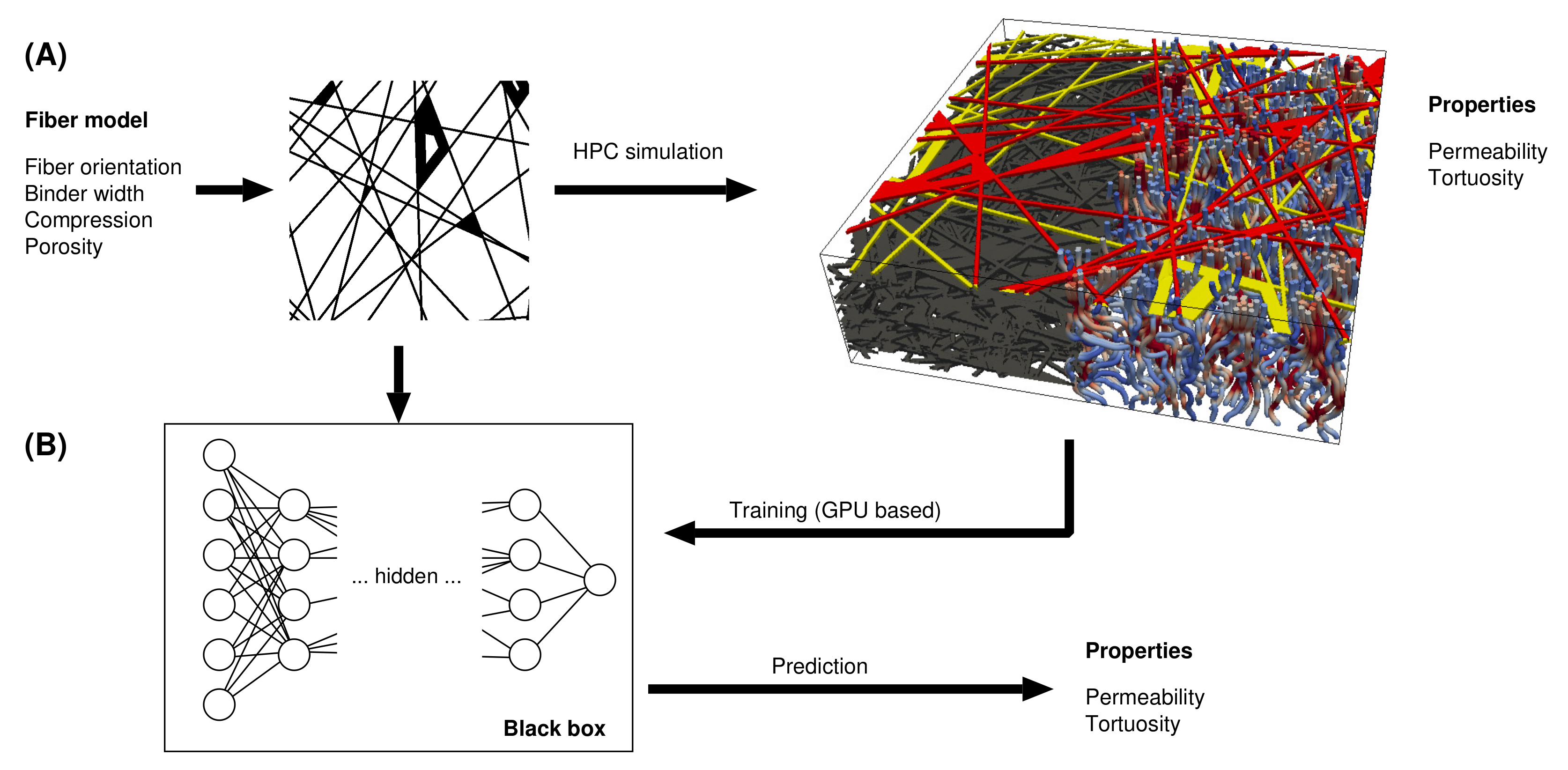
This study investigates the permeability of fiber-based GDLs. The permeabilities of micro-structures generated from a stochastic geometry model were determined in previous LB simulations [9], as depicted in Figure 1. Not only the arrangement of fibers but also the distribution of binders was varied. Furthermore, the underlying micro-structures were compressed. The set of simulation results were then used to train a CNN to predict permeability from the image series. In a similar way, Cawte and Bazylak [32] developed a CNN for the prediction of GDL permeability, with its data generated by pore network modeling (PNM). The relevance of the GDL characteristics as a function of binder and compression was recently analyzed by Wang et al. [33].
Whereas the earlier work of the authors [9,10,34] is based on physical modeling, using the LB method, the present study is data-driven: given the raw data—in this case, the micro-structure of a fiber-based GDL—and its characterization (here, permeability), an ML model is developed to predict these characteristics from a given micro-structure, without the need for HPC simulations.
This paper is organized on the basis of DL, as proposed by El-Amir and Hamdy [35]. The method for generating the training data is described in Section 2, as is the proposed ML model. This includes special features of the data, inherent to the micro-structure, one of which affects the architecture of the CNN. Section 3 presents an overview of the data and their preparation for training. The ML model was validated as shown in Section 4. The predictions of the ML model on real data are presented and discussed in Section 5. Finally, the study is summarized in Section 6.
2. Methods and Available Data
2.1. Machine Learning Model—Overview
For predicting the permeabilities and tortuosities of a porous structure given by a series of BW images, a CNN was developed, as shown in Section 2.2. For training the CNN, a set of micro-structures, as previously published [9], was employed. The training data were given by a series of images of dimensions of 512 × 512 each, all of which had an underlying image resolution of 1.5 µm/px. Further details are presented in Section 2.3.
The training was implemented using the CLAIX supercomputer at RWTH Aachen University, taking advantage of its graphic nodes equipped with two ‘Tesla V100 SXM2 32 GB’ graphics cards.
2.2. Convolutional Neural Network Model
The ML model developed to predict the permeability of a fibrous GDL micro-structure is a CNN. It was developed using Tensorflow and Keras tools [36]. The particular hidden layers of the CNN are as follows:
- Three pairs of three-dimensional convolutional (Conv3D) and average pooling layers;
- Two additional Conv3D layers;
- A flattened layer;
- As a second input, the compression level of the represented material was concatenated with the output of the previous layer;
- Two additional dense layers.
The architecture is illustrated in Figure 2. The main input layer is shown on the left-hand side, with the hidden layers attached from left to right. Noticeable layers in Figure 2 include the three-dimensional convolutional layers, marked as Conv3D. The shape of the structures is written on the right of the Conv3D boxes, after the keyword ‘None’. The dimensions begin with 65 × 512 × 512 and one filter from the input layer, after which the dimensions are reduced stepwise down to 8 × 8 × 8, while the number of filters is doubled from one Conv3D layer to its successor. The functional concatenation with the compression level as a second input layer is also embedded in the bottom part of the visualization. The compression level is extended to an array size of 128 to allow matching with the output of the dense layer.
Given the size of the stacks of input images of 65 × 512 × 512, the architecture shown in Figure 2 leads to 9,776,497 trainable parameters, i.e., the weights of the hidden layers. To evaluate the accuracy of the CNN, the mean squared error (MSE) was used:
where is the set of input structures ; aside from these, the compression levels were also included. h is the function represented by the CNN, the real permeability of the input structure , and m is the number of structures in the set . The MSE from Equation (1) is the loss function of the ML model represented by the CNN. In a similar manner, a percentage error can be defined:
The MPE is more convenient from the technical viewpoint of the application of this CNN, as it can be directly compared with the inaccuracies in experiments or modeling approaches.
2.3. Basic Data
The micro-structure of the Toray-GDL is represented by a stochastic geometry model developed by Thiedmann et al. [37] and analyzed for its transport properties by Froning et al. [9]. The geometry model has three characteristic features:
- Fiber orientation;
- Binder width;
- Compression.
The fiber orientation and binder width are parameters of the Thiedmann model [37], and the compression feature was added by Froning et al. [9]. The micro-structures created by a representation of this model can be characterized as folllows:
- Porosity;
- Permeability;
- Tortuosity.
The porosity is a geometric property, with the permeability and tortuosity being obtained from transport simulations using the LB method. It was shown by Froning et al. [9] that the fiber orientation—represented by stochastic-equivalent ensembles of fiber layers—led to a variation in the permeability and tortuosity. The binder width and compression also affect the transport properties. The geometry model was validated against the real structure using 3D synchrotron data [37]. The consistency of the transport simulations was shown by means of the Karman–Cozeny relationship [9,13].
The basic (training) data for the ML model are the image series generated from a stochastic geometry model developed by Thiedmann et al. [37,38], who specified a fiber model of a Toray 090 GDL based on a stochastic analysis of real fibers and added a binder to fill the void space and achieve the porosity of the real material. Their binder model is represented by a width of binders covering parts of the fibers [37]. Figure 3 illustrates the binder model for selected images.
Fibers with a diameter of 7.5 µm were implemented with an image resolution of 1.5 µm/px, which was further simplified by representing a fiber layer with five identical images [37]. This simplicity was advantageous for the generation of micro-structures for LB simulations [9,34] but led to redundancy of the images in the TP direction. This redundancy, in turn, limited the accuracy—on average, by 5.29%—in previous work [39]. Wirtz used only uncompressed data for training. Although he employed data augmentation—mirroring in two directions and also transposing the images—the accuracy remained limited. Redundant images increase the number of trainable parameters in ML without providing additional information. For this reason, the redundancy of the images was broken by introducing the compression level, as defined by Froning et al. [9].
The introduction of the compression as an additional feature of the data required the specification of the compression level as a second input. Only one number was needed for this purpose. In Figure 2, the second input is shown as a vector of size of 128 intended to match the size of the two inputs of the concatenate layer. This representation was selected to keep the diagram of the architecture as simple as possible, as it is a special extension dedicated to the particular redundancy of the uncompressed input data. The data cited in Figure 3 as A, B, C, and D were reported by Froning et al. [9], uncompressed and compressed. Twenty-five realizations of fiber geometries, multiplied by four different binder distributions, leads to 100 geometries representing the uncompressed material. The image data, representing the realization of a stochastic geometry model, were compressed layer-wise: In regular steps, two adjacent images (representing two adjacent fiber layers) were merged in a binary manner, without creating gray level images. In this way, the total number of images was reduced. On the assumption of the same spatial resolution, the new image series represents the compressed material, as illustrated in detail by Froning et al. [9]. Considering the five steps of compression—10%, 20%, 30%, 40%, and 50%—a total of up to 600 geometries could be available. However, the LB simulations did not converge on some of these, especially the more highly compressed ones, as already reported by Froning et al. [9]. In total, 541 geometries were available for training. Embedded in the micro-structure were three structural features, the most prominent of which was the arrangement of the fibers as proposed by Thiedmann et al. [37], which was validated against real 3D structures. A second feature was a binder model. With this, the porosity of the pure fiber structure was filled in order to achieve that of the real material, leaving the binder width as a model parameter [37]. This is illustrated in the images shown in Figure 3. The orientation of the fibers was adjusted to real data on Toray 090 GDLs [9,37]. In this manner, a porosity of 83% was achieved, whereas the real material has a porosity of 78%. The missing 5% were then filled with the binder—also shown in the illustrations in Figure 3 [37]. The binder width br = 6 µm (Figure 3A) is an extreme case, with most of the fibers being covered by binder material. With increasing binder width, the total length of the fibers being covered with the binder is reduced. The other extreme case is the binder width (Figure 3D), where inside a fiber layer some polygons built by crossing fibers are completely filled with binder. The third feature is the compression level based on an approach shown by Froning et al. [9]. A subset of the data—only uncompressed—was previously used by Wirtz [39] to train a more specialized CNN for permeability prediction.
2.4. Lattice Boltzmann Simulations
The LB simulation technique for obtaining the material characteristics of fiber-based porous GDL material has been demonstrated previously [9,10,34]. A series of BW images defines the micro-structure of a porous paper-type GDL. The geometry was described by a stochastic model, and its representations were analyzed by Froning et al. [9,34]. In this study, this method was used to determine the permeability of the Toray 090 GDL represented by a series of BW images, through-plane and in-plane. The permeability was determined by [9] using LB simulations with the D3Q19 scheme, applying fixed velocity conditions. They considered a small buffer region upstream and downstream of the GDL in order to avoid physically meaningless local conditions. Because of the stochastic nature of the fiber directions, the in-plane characteristics only needed to be calculated for one direction. Based on the LB simulations, the dependency of the permeability on the binder model, as well as the compression, was identified.
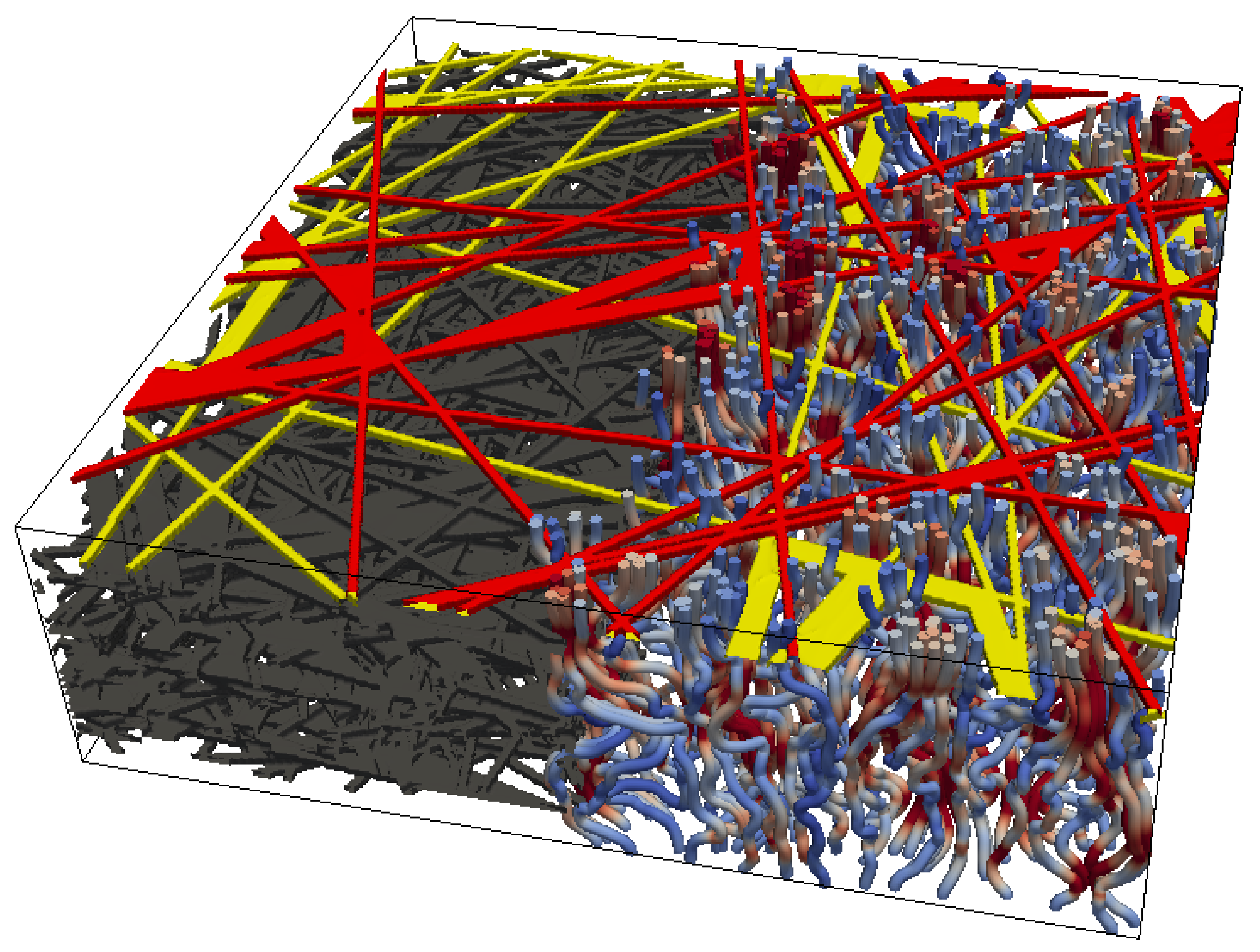
The 3D structure of one of the data points introduced in Section 2.3 is shown in Figure 4. The two top fiber layers are colored in yellow and red to illustrate the irregular geometry. The through-plane simulation (the flow direction is from the bottom to the top) is shown by path lines calculated using the LB method [9]. For better visibility of the flow lines, the micro-structure was faded out from the rightmost half of the domain. The color of the flow lines represent the velocity. The through-plane permeability calculated from the 3D flow field via Darcy’s Law forms the basis of the training data for the proposed ML model. The simulation on compressed material was applied in the same manner after the geometry was modified. For the uncompressed material, each fiber layer was represented by five images, as shown in Figure 3. A compression of 10% was emulated by merging adjacent images of two fiber layers to one, leaving nine images to represent two fiber layers. The compression creates BW images with no gray level ones and was introduced in previous studies [9]. The coarse method of geometry modification led to consistent simulation results for compression of up to 30%. Especially for higher compression, the resulting geometry conflicted with the physics-oriented boundary conditions, and some simulations did not converge. For this reason, only 541 labeled geometries were available for training the ML model instead of 600.
3. Data Preparation
The training constituted the micro-structures from previous investigations [9], based on the stochastic geometry and binder models of Thiedmann et al. [37] and an additional compression approach [9]. They consist of a series of BW images, each with dimensions of 512 × 512. Depending on the amount of compression, the numbers of images in each sample range from 130 (uncompressed) down to 65 in the case of a 50% compression. As the CNN reads structures of a fixed size, all data must be transformed into a common domain size, which was selected as 65 × 512 × 512. The image series of the uncompressed geometry model features five identical BW images for each fiber layer [9]. The compression of the images from 130 to 65 creates images with intermediate gray levels in which some adjacent images were merged using a compression routine. Figure 5 illustrates the intermediate gray level on two sextuples of images following compression. The labels (B) and (D) in Figure 5 relate to the corresponding ones in Figure 3.
4. Validation
The CNN model, trained with the entirety of the data introduced in Section 2.3, was validated according to the five-fold cross-validation method, as presented by El-Amir and Hamdy [35]. In the generic concept of a k-fold cross validation, is often selected as a rule of thumb [35,41]. The extreme value of represents the hold-out validation for resolving a fixed separation of the available data into two sets, namely, training and validation data.
The data were randomly split into five folds, each of the same size. Every fold was picked as a validation set of 20% of the total, taking the other four folds as the training set, or 80% of the total amount of data. The 541 data points were randomly shuffled, then separated into five subsets of size 109, 108, 108, 108, and 108 points. Five folds were defined, each of them incorporating one of the subsets above as a validation set, placing the other four subsets into the training set. The CNN was trained on the training set, after which the MSE was calculated on the validation set, also called the out-of-sample set. With a batch size of 8, the training data (431 or 432 points, respectively) were traversed five times, also known as five epochs. The overall performance of the CNN is the average of the performance values of the individual folds. This raised the computation time for the CNN’s training by a factor of five; however, the estimation of the performance of the CNN to predict the feature—permeability, in this case—is more stable when compared with a training with only one validation set.
The MSE (Equation (1)), applied to the out-of-sample subset of the individual folds, is shown in Table 1. For every fold, the best model parameters were saved during the training, also known as early stopping. The average MSE of the five folds was 0.0643.
The MSE (Equation (1)) was evaluated for the training data, also referred to as the in-sample MSE or training error rate [35]. With long training, there is a risk that the CNN becomes too specialized for the particular training data. It may occur that the MSE, achieved using never-seen data, is worse than the in-sample MSE. Such an effect is referred to as overfitting and can be identified by comparing the in-sample and out-of-sample MSEs. Overfitting would be indicated by a local minimum of the out-of-sample MSE along the training steps. Figure 6 shows the out-of-sample MSE for the five folds. Both the in-sample MSE and out-of-sample MSE are decreasing. For better visibility, the in-sample MSE is only displayed for one fold. The progress of the out-of-sample MSE demonstrates that no overfitting was observed during training. The MSE of fold no. 2 is larger than the others (Table 1). This is also reflected by the red line in Figure 6, specifying the development of the MSE in the five folds: this curve is slightly higher than the others. On the other hand, a peak at the end of the training is shown by folds 4 and 5. Such effects were overcome using the early stopping method during training.
The training of one fold, as summarized in Table 1, required more than one hour on a standard computer equipped with a ‘GeForce GTX 1070 OC 8 GB’ graphics card. On one node of the CLAIX system at RWTH Aachen University, equipped with two ‘Tesla V100 SXM2 32 GB’ graphic cards, the same training was performed in less than nine minutes.
5. Results and Discussion
The results of the ML model were evaluated according to several parameters. The accuracy of the prediction permeability of the training and validation data by the trained CNN is first presented.
As described in Section 3, the ML model was trained on a series of 65 images with 512 × 512 dimensions. These were compressed in the through-plane direction in order to cover both uncompressed and compressed images. In the uncompressed format, these images represent a structure sized 130 × 512 × 512.
The prediction of the permeability of the Toray 090 data introduced in Section 2.3 represents the foreseen application of the proposed CNN: a series of images of fixed size, and the same image resolution of 1.5 µm/px.
The accuracy of the predictions shown in Table 2 is below 5.11% in all cases, and in the percentile range for the relevant cases with a binder with br < 30 µm. This is superior to many of the experimental data, as reported by Hussaini et al. [42]. It is also within the accuracy of LB simulations, given that such simple coarse grids represent the micro-structure [9,34]. The CNN was trained to make predictions based on micro-structures and their respective compression levels. As noted in Section 2.3, there is a hidden feature—the binder model—embedded in the micro-structure. Without preference for any fold of the cross-validation introduced in Section 4, the last one (No. 5) was selected for further analysis. Although the MSE (Equation (1)) was specified as a loss function for the CNN training, the MPE (Equation (2)) is more convenient for addressing the theoretical viewpoint. Table 2 displays the predicted permeability that was averaged over subsets of particular compression levels and binder widths . Moreover, the averaged MPE and MSE are given. The MPE was not homogeneously distributed with respect to the features binder width and compression level. In Table 2, the influence of the features is depicted by the quantiles of permeability, which are dramatically reduced with increasing compression. This effect can be observed for every binder width . A reduction in the permeability with increasing binder width of the binder model can also be observed in Table 2. In this case, the permeabilities of the selected compression levels were compared together with the binder width. In comparison to the compression level, the impact of the binder width is less pronounced. The number of data points—less than or equal to 25—is given for each combination of compression level and binder width. Numbers of less than 25 indicate numerical deficits in the previous LB simulations that were already noticed in earlier investigations [9]. This effect tends to emerge at high compression levels and extreme binder widths . The highest compression level of 50% generally has a low level of accuracy in terms of prediction by the CNN. On the one hand, this is the worst-case scenario of the simplified compression algorithm developed earlier [9]. On the other hand, it was found that paper-type GDLs are usually compressed by up to 30% when they are assembled in a fuel cell stack. Hoppe et al. [1] compressed their GDLs by up to 30%, whereas Nitta et al. [43] investigated compressions of up to 40%.
The interquartile range (IQR) is the difference between the 75% and 25% quantiles, also known as the third and first quartiles. The IQR is larger than 1 µm2 in most cases but larger than 0.5 µm2 in cases of low permeability, i.e., with medians smaller than 10 µm2. This applies to at least the relevant compression levels of up to 30%. The variation in the permeability caused by the micro-structure—indicated by the IQR—is larger than the MPE presented in Table 2.
The large variation in the permeability within one group (binder with compression) shown in Table 2 represents the inhomogeneity of the porous material. An increasing width of the binder (Figure 3) increases the local areas blocking the fluid flow through the micro-structure. The inhomogeneity of the fluid flow is illustrated in Figure 4. The permeability decreases under compression in accordance with the Karman–Cozeny relationship [9].
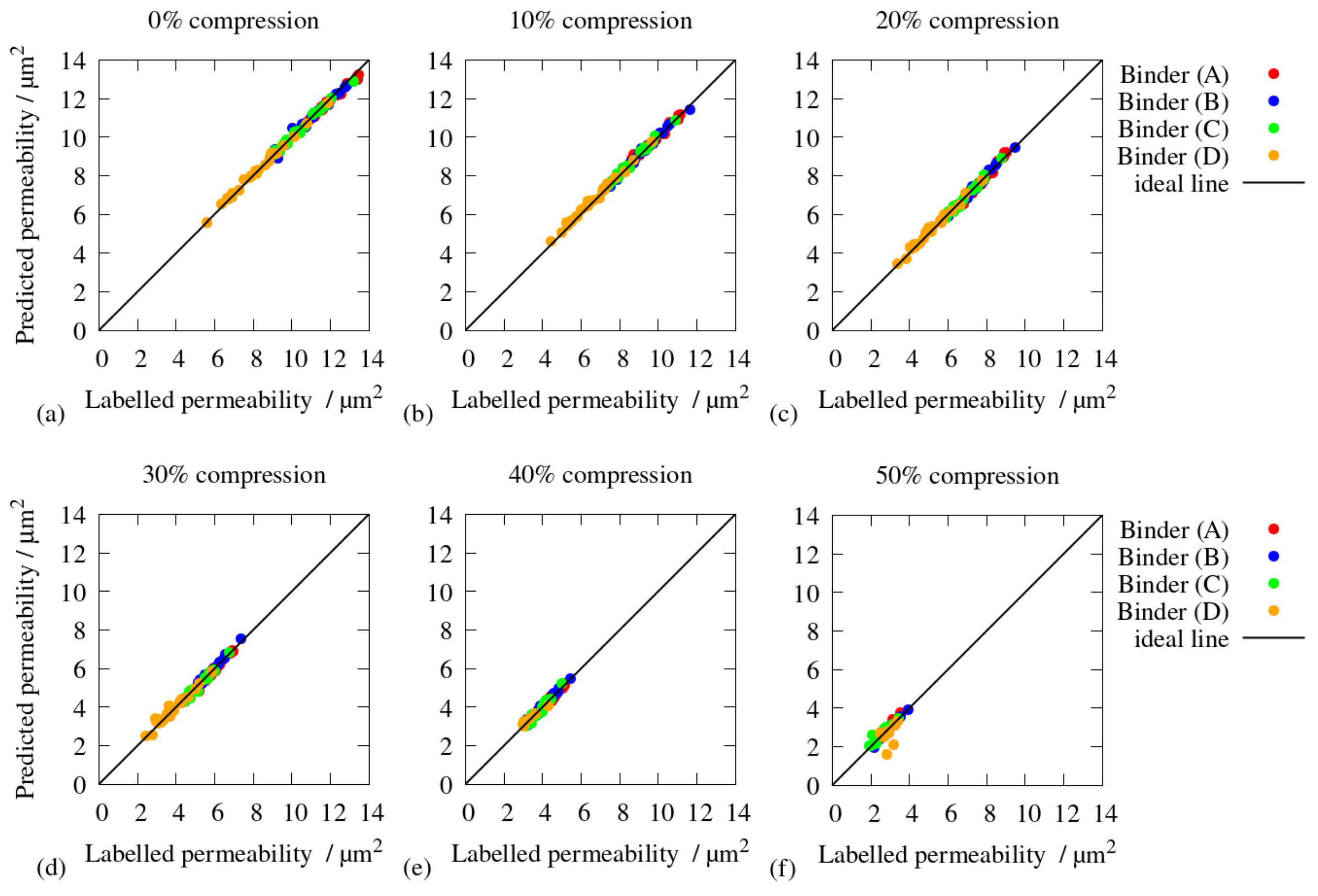
Figure 7 displays the accuracy of the permeabilities predicted by the CNN on the training and validation data, separated by the compression level. The predicted values (the y-axis in the diagrams) are compared with the correct values previously calculated using LB simulations. In addition, the values are colored according to the binder model. Although this feature was not entered into the CNN, the clusters are represented by the ML model, as they were already previously identified by Froning et al. [9]. Along with higher grades of compression, the permeabilities decrease, which is in accordance with Tomadakis et al. [13], our previous investigations [9], and the experimental results of Feser et al. [44] and Hoppe [45]. As proposed by Froning et al. [9], the compressed data exhibit systematically lower permeabilities than the uncompressed data. Nevertheless, Froning et al. [9] state that the binder model with br = 18 µm is the most realistic one compared with the real material. In particular, the high compression level of 50% exhibits a lower degree of accuracy than the others. On the other hand, the high compression levels suffer from inaccuracies as a result of how they were constructed. The most inaccurate data, with 50% compression, were also found to be unrealistic in previous investigations [9].
Figure 8 shows the accuracy of the CNN predictions applied to the validation data, colored according to the binder model. The diagram illustrates that the prediction by the CNN is best for the binder models with br ≤ 30 µm, which are more realistic than the other two variants [9]. The parameter for the binder width was originally introduced by Thiedmann et al. [38] to model the distribution of the binder along the fibers of the GDL. They presented variant as an extreme case. This is illustrated in Figure 3D, in which polygons built by fibers were fully filled with binder material. Due to the stochastic nature of the fiber arrangement, such areas can be large, as in Figure 5D. In these cases, the gas flow would be dramatically inhibited, causing a different flow behavior than in micro-structures with limited binder widths.
The quantiles shown in Table 2 and the deviations of the predicted permeability from the LB simulations presented in Figure 7 and Figure 8 indicate that the accuracy of the predictions of the CNN is smaller than the variation of the permeability caused by the stochastic geometry model.
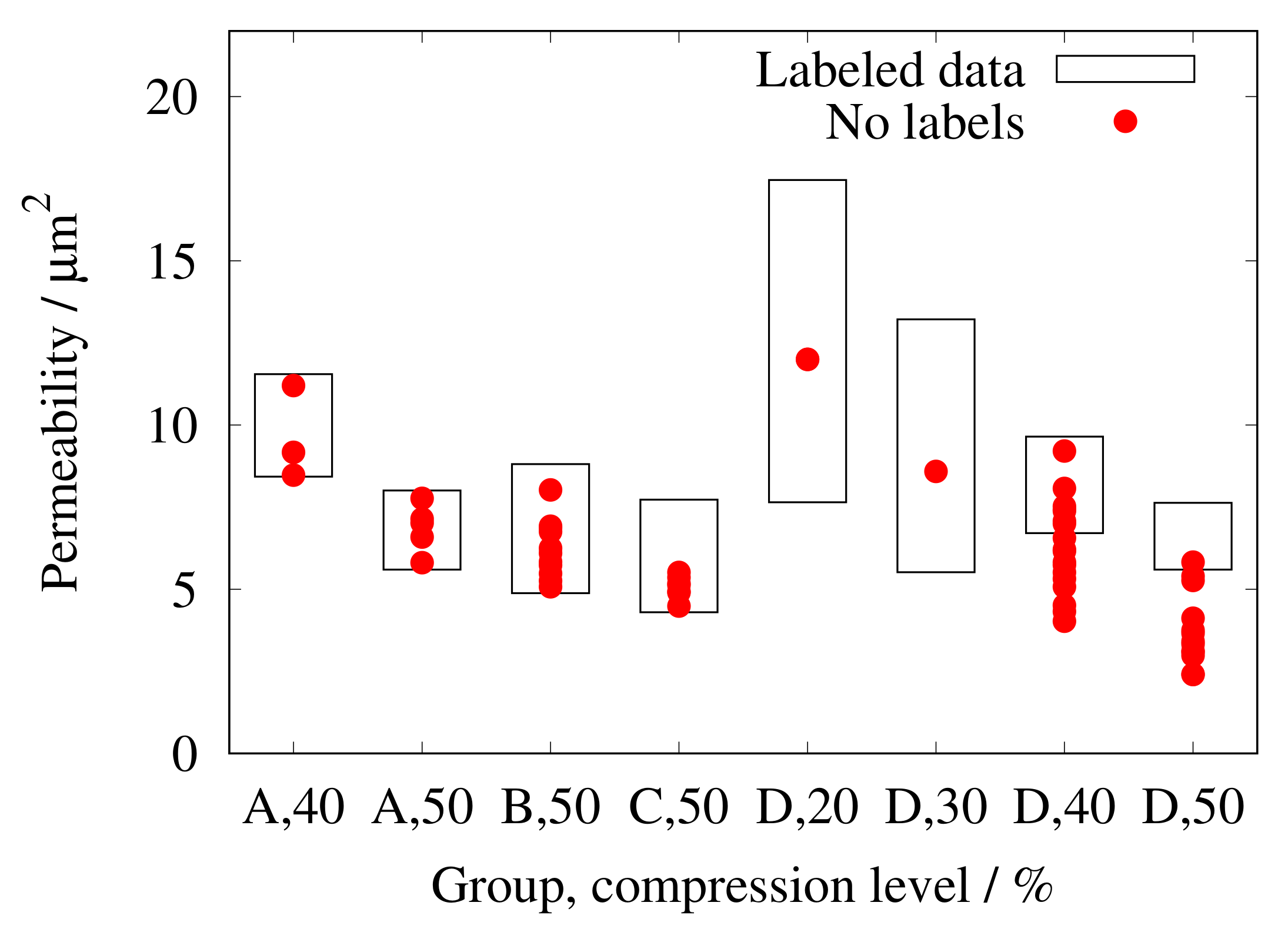
As noted in Section 2.4, only 541 simulations of the 600 available data-sets led to a physically consistent result. The permeabilities of the micro-structures of the other 59 virtual geometries were predicted by the ML model. Figure 9 displays the groups of the binder model (Figure 3) and compression level. The minimum and maximum values of the LB simulations within the particular groups of data are shown as boxes. Each group of data consists of 25 image series, with numbers of unlabeled data in the groups as follows: three in group A, 40%; five in group A, 50%; eleven in group B, 50%; seven in group C, 50%; one in group D, 20%; one in group D, 30%; eighteen in group D, 40%; and thirteen in group D, 50%. In most of the groups, the predicted permeability of unlabeled micro-structures was within the range of permeabilities calculated earlier by the LB simulation, except for groups D, with 40% and 50%. The latter group suffers from having only being subject to a few successful simulations by Froning et al. [9]. The wider range of predicted permeabilities results from the small amount of labeled data in these two groups. This indicates that the CNN is able to predict consistent permeability values for micro-structures that are not eligible for LB simulations as soon as the material is within the feature range of the training data. In a similar manner, Yuan et al. [25] filled missing positions in their membrane database with ML-predicted values.
The results show that a CNN is able to accurately predict the permeability of GDLs, with a limited number of geometries used for training. The training data were created by means of a stochastic geometry model that had been validated in previous investigations [9]. The CNN was trained with labeled permeabilities. Additional features—compression level and the binder model—are inherent in the training data but were not labeled in the training phase. With increasing compression, the permeability predicted by the CNN systematically decreases. Moreover, the binder model exhibits a systematic influence on the permeability. Both effects were also reported in previous investigations using the LB method [9,34]. The impact of these two parameters on the predicted permeability is larger than the deviation of the predicted permeability from that computed with the LB method.
6. Conclusions
In this paper, it was shown that permeability can be predicted by a CNN with an accuracy that is smaller than the statistical variance produced by the stochastic geometry model. Inherent features—binder type and compression of the material—were reproduced by the ML prediction. Data that were not successfully analyzed by transport simulations in previous studies could be processed by the ML model with consistent results. The trained CNN can be applied to image series representing a micro-structure of the same kind as the training data. The calculation of the permeability using transport simulations in the micro-structure requires HPC resources. It was found that the training of the CNN also necessitates these. Predictions of the permeability of the particular micro-structure, however, can be performed on a standard desktop computer. The demonstrated ML methods make the calculation of material characteristics available to a wider community. The method can be extended to train characteristics in addition to permeability. Furthermore, different kinds of micro-structures can be added to the training data, as long as the characteristics can be provided.
Author Contributions
Conceptualization, D.F. and E.H.; formal analysis, D.F.; methodology, J.W.; investigation and software, J.W.; validation, D.F. and J.W.; writing, D.F.; supervision, W.L. All authors have read and agreed to the published version of the manuscript.
Funding
This research was funded by the Deutsche Forschungsgemeinschaft (DFG, German Research Foundation)—491111487.
Institutional Review Board Statement
Not applicable.
Informed Consent Statement
Not applicable.
Data Availability Statement
Not applicable.
Acknowledgments
The authors gratefully acknowledge the computation time granted by the JARA Vergabegremium and provided in the JARA Partition portion of the supercomputer JURECA at the Forschungszentrum Jülich and on the JARA Partition section of the CLAIX supercomputer at RWTH Aachen University. We thank Christopher Wood for proofreading the manuscript.
Conflicts of Interest
The authors declare no conflict of interest.
References
- Hoppe, E.; Janßen, H.; Müller, M.; Lehnert, W. The impact of flow field plate misalignment on the gas diffusion layer intrusion and performance of a high-temperature polymer electrolyte fuel cell. J. Power Sources 2021, 501, 230036. [Google Scholar] [CrossRef]
- Kvesić, M.; Reimer, U.; Froning, D.; Lüke, L.; Lehnert, W.; Stolten, D. 3D modeling of a 200 cm2 HT-PEFC short stack. Int. J. Hydrogen Energy 2012, 37, 2430–2439. [Google Scholar] [CrossRef]
- Reimer, U.; Nikitsina, E.; Janßen, H.; Müller, M.; Froning, D.; Beale, S.B.; Lehnert, W. Design and Modeling of Metallic Bipolar Plates for a Fuel Cell Range Extender. Energies 2021, 14, 5484. [Google Scholar] [CrossRef]
- Mukherjee, M.; Bonnet, C.; Lapique, F. Estimation of through-plane and in-plane gas permeability across gas diffusion layers (GDLs): Comparison with equivalent permeability in bipolar plates and relation to fuel cell performance. Int. J. Hydrogen Energy 2020, 45, 13428–13440. [Google Scholar] [CrossRef]
- Yuan, X.Z.; Nayoze-Coynel, C.; Shaigan, N.; Fisher, D.; Zhao, N.; Zamel, N.; Gazdzicki, P.; Ulsh, M.; Friedrich, K.A.; Girard, F.; et al. A review of functions, attributes, properties and measurements for the quality control of proton exchange membrane fuel cell components. J. Power Sources 2021, 491, 229540. [Google Scholar] [CrossRef]
- Yuan, X.Z.; Li, H.; Gu, E.; Qian, W.; Girard, F.; Wang, Q.; Biggs, T.; Jaeggle, M. Measurements of GDL Properties for Quality Control in Fuel Cell Mass Production Line. World Electr. Veh. J. 2016, 8, 422–430. [Google Scholar] [CrossRef] [Green Version]
- Kaneko, H.; Ohta, K.; Shimuzu, M.; Araki, T. Measurements of Anisotropy of the Effective Diffusivity through PEFC GDL and Mass Transfer Resistance at GDL and Channel Interface. Trans. Jpn. Soc. Mech. Eng. Ser. B 2013, 79, 71–81. [Google Scholar] [CrossRef] [Green Version]
- Syarif, N.; Rohendi, D.; Nanda, A.D.; Sandi, M.T.; Sihombing, D.S.W.B. Gas diffusion layer from Binchotan carbon and its electrochemical properties for supporting electrocatalyst in fuel cell. AIMS Energy 2022, 10, 292–305. [Google Scholar] [CrossRef]
- Froning, D.; Brinkmann, J.; Reimer, U.; Schmidt, V.; Lehnert, W.; Stolten, D. 3D analysis, modeling and simulation of transport processes in compressed fibrous microstructures, using the Lattice Boltzmann method. Electrochim. Acta 2013, 110, 325–334. [Google Scholar] [CrossRef] [Green Version]
- Froning, D.; Yu, J.; Gaiselmann, G.; Reimer, U.; Manke, I.; Schmidt, V.; Lehnert, W. Impact of compression on gas transport in non-woven gas diffusion layers of high temperature polymer electrolyte fuel cells. J. Power Sources 2016, 318, 26–34. [Google Scholar] [CrossRef]
- Zhang, H.; Zhu, L.; Harandi, H.B.; Duan, K.; Zeis, R.; Sui, P.C.; Chuang, P.Y.A. Microstructure reconstruction of the gas diffusion layer and analyses of the anisotropic transport properties. Energy Convers. Manag. 2021, 241, 114293. [Google Scholar] [CrossRef]
- Gao, Y.; Jin, T.; Wu, X. Stochastic 3D Carbon Cloth GDL Reconstruction and Transport Prediction. Energies 2020, 13, 572. [Google Scholar] [CrossRef] [Green Version]
- Tomadakis, M.M.; Robertson, T.J. Viscous Permeability of Random Fiber Structures: Comparison of Electrical and Diffusional Estimates with Experimental and Analytical Results. J. Compos. Mater. 2005, 39, 163–188. [Google Scholar] [CrossRef]
- Lee, S.-H.; Nam, J.H.; Kim, C.J.; Kim, H.M. Effect of fiber orientation on Liquid–Gas flow in the gas diffusion layer of a polymer electrolyte membrane fuel cell. Int. J. Hydrogen Energy 2021, 46, 33957–33968. [Google Scholar] [CrossRef]
- Lintermann, A.; Schröder, W. Lattice–Boltzmann simulations for complex geometries on high-performance computers. CEAS Aeronaut. J. 2020, 11, 745–766. [Google Scholar] [CrossRef]
- Chollet, F. Deep Learning with Python; Manning: Shelter Island, NJ, USA, 2017; ISBN 9781617294433. [Google Scholar]
- Oliveira, O.N.; Beljonne, D.; Wong, S.S.; Schanze, K.S. Forum on Artificial Intelligence/Machine Learning for Design and Development of Applied Materials. ACS Appl. Mater. Interfaces 2021, 13, 53301–53302. [Google Scholar] [CrossRef]
- Zhao, J.; Qin, F.; Derome, D.; Carmeliet, J. Simulation of quasi-static drainage displacement in porous media on pore-scale: Coupling lattice Boltzmann method and pore network model. J. Hydrol. 2020, 588, 125080. [Google Scholar] [CrossRef]
- Kamrava, S.; Tahmasebi, P.; Sahimi, M. Linking Morphology of Porous Media to Their Macroscopic Permeability by Deep Learning. Transp. Porous Media 2019, 131, 427–448. [Google Scholar] [CrossRef]
- Ishola, O.; Vilcáez, J. Machine learning modeling of permeability in 3D heterogeneous porous media using a novel stochastic pore-scale simulation approach. Fuel 2022, 321, 124044. [Google Scholar] [CrossRef]
- Graczyk, K.M.; Matyka, M. Predicting porosity, permeability, and tortuosity of porous media from images by deep learning. Sci. Rep. 2020, 10, 21488. [Google Scholar] [CrossRef] [PubMed]
- Yasuda, T.; Ookawara, S.; Yoshikawa, S.; Matsumoto, H. Machine learning and data-driven characterization framework for porous materials: Permeability prediction and channeling defect detection. Chem. Eng. J. 2021, 420, 130069. [Google Scholar] [CrossRef]
- Rao, C.; Liu, Y. Three-dimensional convolutional neural network (3D-CNN) for heterogeneous material homogenization. Comput. Mater. Sci. 2020, 184, 109850. [Google Scholar] [CrossRef]
- Wan, S.; Liang, X.; Jiang, H.; Sun, J.; Djilali, N.; Zhao, T. A coupled machine learning and genetic algorithm approach to the design of porous electrodes for redox flow batteries. Appl. Energy 2021, 298, 117177. [Google Scholar] [CrossRef]
- Yuan, Q.; Longo, M.; Thornton, A.W.; McKeown, N.B.; Comesaña-Gándara, B.; Jansen, J.C.; Jelfs, K.E. Imputation of missing gas permeability data for polymer membranes using machine learning. J. Membr. Sci. 2021, 627, 119207. [Google Scholar] [CrossRef]
- Tahmasebi, P.; Kamrava, S.; Bai, T.; Sahimi, M. Machine learning in geo- and environmental sciences: From small to large scale. Adv. Water Resour. 2020, 142, 103619. [Google Scholar] [CrossRef]
- Kamrava, S.; Sahimi, M.; Tahmasebi, P. Simulating fluid flow in complex porous materials by integrating the governing equations with deep-layered machines. npj Comput. Mater. 2021, 7, 127. [Google Scholar] [CrossRef]
- Wang, Y.; Seo, B.; Wang, B.; Zamel, N.; Jiao, K.; Adroher, X.C. Fundamentals, materials, and machine learning of polymer electrolyte membrane fuel cell technology. Energy AI 2020, 1, 100014. [Google Scholar] [CrossRef]
- Colliard-Granero, A.; Batool, M.; Jankovic, J.; Jitsev, J.; Eikerling, M.H.; Malek, K.; Eslamibidgoli, M.J. Deep learning for the automation of particle analysis in catalyst layers for polymer electrolyte fuel cells. Nanoscale 2022, 14, 10–18. [Google Scholar] [CrossRef] [PubMed]
- Hwang, H.; Ahn, J.; Lee, H.; Oh, J.; Kim, J.; Ahn, J.P.; Kim, H.K.; Lee, J.H.; Yoon, Y.; Hwang, J.H. Deep learning-assisted microstructural analysis of Ni/YSZ anode composites for solid oxide fuel cells. Mater. Charact. 2021, 172, 110906. [Google Scholar] [CrossRef]
- Bührer, M.; Xu, H.; Hendriksen, A.A.; Büchi, F.N.; Eller, J.; Stampanoni, M.; Marone, F. Deep learning based classification of dynamic processes in time-resolved X-ray tomographic microscopy. Sci. Rep. 2021, 11, 24174. [Google Scholar] [CrossRef] [PubMed]
- Cawte, T.; Bazylak, A. A 3D convolutional neural network accurately predicts the permeability of gas diffusion layer materials directly from image data. Curr. Opin. Electrochem. 2022, 35, 101101. [Google Scholar] [CrossRef]
- Wang, H.; Yang, G.; Li, S.; Shen, Q.; Liao, J.; Jiang, Z.; Zhang, G.; Zhang, H.; Su, F. Effect of Binder and Compression on the Transport Parameters of a Multilayer Gas Diffusion Layer. Energy Fuels 2021, 35, 15058–15073. [Google Scholar] [CrossRef]
- Froning, D.; Gaiselmann, G.; Reimer, U.; Brinkmann, J.; Schmidt, V.; Lehnert, W. Stochastic Aspects of Mass Transport in Gas Diffusion Layers. Transp. Porous Media 2014, 103, 469–495. [Google Scholar] [CrossRef]
- El-Amir, H.; Hamdy, M. Deep Learning Pipeline; Apress: Berkeley, CA, USA, 2020. [Google Scholar] [CrossRef]
- Géron, A. Hands-On Machine Learning with Scikit-Learn, Keras, and TensorFlow. Concepts, Tools, and Techniques to Build Intelligent Systems, 2nd ed.; O’Reilly: Sebastopol, CA, USA, 2019; ISBN 978-1-49203264-9. [Google Scholar]
- Thiedmann, R.; Fleischer, F.; Hartnig, C.; Lehnert, W.; Schmidt, V. Stochastic 3D Modeling of the GDL Structure in PEMFCs Based on Thin Section Detection. J. Electrochem. Soc. 2008, 155, B391–B399. [Google Scholar] [CrossRef]
- Thiedmann, R.; Hartnig, C.; Manke, I.; Schmidt, V.; Lehnert, W. Local Structural Characteristics of Pore Space in GDLs of PEM Fuel Cells Based on Geometric 3D Graphs. J. Electrochem. Soc. 2009, 156, B1339. [Google Scholar] [CrossRef]
- Wirtz, J. Untersuchung von Neuronalen Architekturen für ein Prediktives Modell der Eigenschaften von Faserbasierten Gasdiffusionsschichten. Bachelor’s Thesis, University of Applied Sciences, Aachen, Germany, 2021. [Google Scholar]
- Centre, J.S. JURECA: Modular supercomputer at Jülich Supercomputing Centre. J. Large-Scale Res. Facil. 2018, 4, A132. [Google Scholar]
- Pillonetto, G.; Dinuzzo, F.; Chen, T.; Nicolao, G.D.; Ljung, L. Kernel methods in system identification, machine learning and function estimation: A survey. Automatica 2014, 50, 657–682. [Google Scholar] [CrossRef] [Green Version]
- Hussaini, I.S.; Wang, C.Y. Measurement of relative permeability of fuel cell diffusion media. J. Power Sources 2010, 195, 3830–3840. [Google Scholar] [CrossRef]
- Nitta, I.; Hottinen, T.; Himanen, O.; Mikkola, M. Inhomogeneous compression of PEMFC gas diffusion layer. J. Power Sources 2007, 171, 26–36. [Google Scholar] [CrossRef]
- Feser, J.; Prasad, A.; Advani, S. Experimental characterization of in-plane permeability of gas diffusion layers. J. Power Sources 2006, 162, 1226–1231. [Google Scholar] [CrossRef]
- Hoppe, E. Kompressionseigenschaften der Gasdiffusionslage einer Hochtemperatur-Polymerelektrolyt-Brennstoffzelle. Ph.D. Thesis, RWTH Aachen University, Aachen, Germany, 2021. [Google Scholar]
Figure 1.
Data scheme. (A) Historical data from Froning et al. [9]; (B) ML approach in the manuscript.
Figure 1.
Data scheme. (A) Historical data from Froning et al. [9]; (B) ML approach in the manuscript.

Figure 2.
Architecture of the CNN representing the proposed ML model.

Figure 3.
Binder applied to fiber representations using four different radii : (A) = , (B) = , (C) = , and (D) .
Figure 3.
Binder applied to fiber representations using four different radii : (A) = , (B) = , (C) = , and (D) .

Figure 4.
The 3D structure of a micro-structure with = and through-plane transport simulation [9].
Figure 4.
The 3D structure of a micro-structure with = and through-plane transport simulation [9].

Figure 5.
Image compression of two examples of consecutive images. Six BW images were compressed into three gray level images; (B) images 3–8 of a stack with = ; (D) images 3–8 of a stack with ; see Figure 3.
Figure 5.
Image compression of two examples of consecutive images. Six BW images were compressed into three gray level images; (B) images 3–8 of a stack with = ; (D) images 3–8 of a stack with ; see Figure 3.

Figure 6.
Development of the MSE during training.

Figure 7.
Predictions on the training and validation data, colored according to the binder width ; see Figure 3; (a) uncompressed; (b) 10% compression; (c) 20% compression; (d) 30% compression; (e) 40% compression; (f) 50% compression.
Figure 7.
Predictions on the training and validation data, colored according to the binder width ; see Figure 3; (a) uncompressed; (b) 10% compression; (c) 20% compression; (d) 30% compression; (e) 40% compression; (f) 50% compression.

Figure 8.
Predictions on the out-of-sample data; coloring according to the binder model: (A) br = 66 µm; (B) br = 18 µm; (C) br = 30µm; (D) br = ∞.
Figure 8.
Predictions on the out-of-sample data; coloring according to the binder model: (A) br = 66 µm; (B) br = 18 µm; (C) br = 30µm; (D) br = ∞.

Figure 9.
Predictions on unlabeled data, compared with the minimum and maximum values of the same group of labeled data.
Figure 9.
Predictions on unlabeled data, compared with the minimum and maximum values of the same group of labeled data.


Table 1.
Performance of the CNN on the individual folds. The MSE was calculated for the out-of-sample subset using the smallest MSE (early stopping).
Table 1.
Performance of the CNN on the individual folds. The MSE was calculated for the out-of-sample subset using the smallest MSE (early stopping).
| Training Set 80%, Test Set 20% | ||||||
|---|---|---|---|---|---|---|
| Fold | Out of Sample = X | MSE | ||||
| 1 | X | 0.0676 | ||||
| 2 | X | 0.1128 | ||||
| 3 | X | 0.0389 | ||||
| 4 | X | 0.0446 | ||||
| 5 | X | 0.0578 | ||||
| Average | 0.0643 | |||||
Table 2.
Predicted permeability, mean percentage error MPE, and mean squared error MSE on subsets of training and validation data of Fold No. 5.
Table 2.
Predicted permeability, mean percentage error MPE, and mean squared error MSE on subsets of training and validation data of Fold No. 5.
| Comp. | No. | Quantiles of Predicted Permeability/ | MPE/% | MSE/ | |||||||
|---|---|---|---|---|---|---|---|---|---|---|---|
| / | /% | min | 25% | 50% | 75% | Max | Training | Validation | Training | Validation | |
| 6 | 0 | 25 | 10.42 | 11.04 | 11.55 | 12.17 | 13.23 | 0.88 | 0.92 | 0.024 | 0.016 |
| 10 | 25 | 8.62 | 9.20 | 9.56 | 10.14 | 11.19 | 0.73 | 2.77 | 0.007 | 0.077 | |
| 20 | 25 | 6.56 | 7.22 | 7.60 | 8.16 | 9.22 | 1.10 | 1.58 | 0.012 | 0.023 | |
| 30 | 25 | 4.81 | 5.39 | 5.72 | 6.21 | 6.94 | 1.09 | 2.66 | 0.007 | 0.038 | |
| 40 | 22 | 3.60 | 3.95 | 4.30 | 4.53 | 5.25 | 2.08 | 1.81 | 0.010 | 0.009 | |
| 50 | 20 | 2.38 | 2.73 | 2.85 | 3.18 | 3.78 | 2.15 | 5.37 | 0.007 | 0.033 | |
| 18 | 0 | 25 | 8.91 | 10.52 | 11.10 | 11.70 | 13.38 | 0.85 | 2.43 | 0.013 | 0.115 |
| 10 | 25 | 7.46 | 8.71 | 9.15 | 9.65 | 11.44 | 0.90 | 1.99 | 0.010 | 0.036 | |
| 20 | 25 | 5.87 | 6.85 | 7.14 | 7.66 | 9.44 | 1.05 | 1.76 | 0.008 | 0.017 | |
| 30 | 25 | 4.32 | 5.25 | 5.42 | 5.84 | 7.53 | 1.34 | 1.83 | 0.010 | 0.011 | |
| 40 | 25 | 3.08 | 3.71 | 4.01 | 4.31 | 5.47 | 1.73 | 2.96 | 0.007 | 0.016 | |
| 50 | 14 | 1.97 | 2.49 | 2.70 | 3.02 | 3.93 | 1.69 | 4.06 | 0.005 | 0.015 | |
| 30 | 0 | 25 | 9.10 | 9.66 | 10.24 | 11.32 | 12.87 | 0.89 | 0.82 | 0.015 | 0.009 |
| 10 | 25 | 7.48 | 7.91 | 8.38 | 9.35 | 10.85 | 0.93 | 1.37 | 0.010 | 0.016 | |
| 20 | 25 | 5.84 | 6.24 | 6.49 | 7.39 | 8.92 | 1.02 | 1.50 | 0.008 | 0.013 | |
| 30 | 25 | 4.28 | 4.72 | 4.85 | 5.51 | 6.84 | 1.62 | 2.70 | 0.010 | 0.028 | |
| 40 | 25 | 3.02 | 3.39 | 3.61 | 4.09 | 5.21 | 2.07 | 4.05 | 0.008 | 0.032 | |
| 50 | 18 | 2.06 | 2.35 | 2.60 | 2.89 | 3.47 | 3.68 | 9.58 | 0.014 | 0.077 | |
| ∞ | 0 | 25 | 5.57 | 7.23 | 8.11 | 9.12 | 11.78 | 1.17 | 1.41 | 0.012 | 0.021 |
| 10 | 25 | 4.60 | 5.86 | 6.67 | 7.35 | 9.73 | 1.92 | 4.10 | 0.019 | 0.052 | |
| 20 | 24 | 3.48 | 4.46 | 5.15 | 5.75 | 7.76 | 2.50 | 1.63 | 0.022 | 0.011 | |
| 30 | 24 | 2.49 | 3.33 | 3.90 | 4.28 | 5.85 | 3.90 | 4.26 | 0.032 | 0.048 | |
| 40 | 7 | 3.02 | 3.16 | 3.28 | 3.52 | 4.05 | 3.36 | 3.69 | 0.018 | 0.031 | |
| 50 | 12 | 1.61 | 2.56 | 2.71 | 2.76 | 3.33 | 5.11 | 38.35 | 0.025 | 1.319 | |
Publisher’s Note: MDPI stays neutral with regard to jurisdictional claims in published maps and institutional affiliations. |
© 2022 by the authors. Licensee MDPI, Basel, Switzerland. This article is an open access article distributed under the terms and conditions of the Creative Commons Attribution (CC BY) license (https://creativecommons.org/licenses/by/4.0/).
Share and Cite
MDPI and ACS Style
Froning, D.; Wirtz, J.; Hoppe, E.; Lehnert, W. Flow Characteristics of Fibrous Gas Diffusion Layers Using Machine Learning Methods. Appl. Sci. 2022, 12, 12193. https://doi.org/10.3390/app122312193
AMA Style
Froning D, Wirtz J, Hoppe E, Lehnert W. Flow Characteristics of Fibrous Gas Diffusion Layers Using Machine Learning Methods. Applied Sciences. 2022; 12(23):12193. https://doi.org/10.3390/app122312193
Chicago/Turabian StyleFroning, Dieter, Jannik Wirtz, Eugen Hoppe, and Werner Lehnert. 2022. "Flow Characteristics of Fibrous Gas Diffusion Layers Using Machine Learning Methods" Applied Sciences 12, no. 23: 12193. https://doi.org/10.3390/app122312193
Note that from the first issue of 2016, this journal uses article numbers instead of page numbers. See further details here.